(The Final) CountdownJean-Marc Alliot* |
Abstract: The Countdown game is one of the oldest TV show running in the world. It started broadcasting in 1972 on the french television and in 1982 on British channel 4, and it has been running since in both countries. The game, while extremely popular, never received any serious scientific attention, probably because it seems too simple at first sight. We present in this article an in-depth analysis of the numbers round of the countdown game. This includes a complexity analysis of the game, an analysis of existing algorithms, the presentation of a new algorithm that increases resolution speed by a factor of 20. It also includes some leads on how to turn the game into a more difficult one, both for a human player and for a computer, and even to transform it into a probably undecidable problem.
The Countdown (Wikipedia [2015]) game is one of the oldest TV show running in the world. It started broadcasting in 1972 on the french television as “des chiffres et des lettres”, literally “numbers and letters” with a numbers round called “Le compte est bon”, literally “the count is good”). It started broadcasting in 1982 on British channel 4 as “Countdown”, and it has been running since in both countries.
The numbers round of the game is extremely simple: 6 numbers are drawn from a set of 24 which contains all numbers from 1 to 10 (small numbers) twice plus 25, 50, 75 and 100 (large numbers). Then, with these six numbers, the contestants have to find a number randomly drawn between 101 and 9991, or, if it is impossible, the closest number to the number drawn. Only the four standard operations (+ − × /) can be used. As soon as two numbers have been used to make a new one, they can’t be used again, but the new number found can be used. For example, if the six numbers drawn are 1,1,4,5,6,7 and the number to find is 899 the answer is:
  Operations   Remaining
 6 x  5 = 30  {1,1,4,7,30}
30 +  1 = 31  {1,4,7,31}
 4 x  7 = 28  {1,28,31}
28 +  1 = 29  {29,31}
29 * 31 = 899 {899}
There are usually different ways to find a solution. The simplest answer is usually defined as the answer using the least number of operations, and if two solutions have the same number of operations, a possible refinement is to keep the one having the smallest highest number2.
The game, while extremely popular, never received any serious scientific attention. There was a very early article in the french magazine “l’Ordinateur Individuel” in the late seventies, written by Jean-Christophe Buisson (Buisson [1980]), which described a simple algorithm. The only article written on the subject in English was published twice (Defays [1990], Defays [1995a]) by Daniel Defays. Defays also published in 1995 a book in french (Defays [1995b]) which used the game as a central example for introducing artificial intelligence methods. But the ultimate goal of Defays was not to develop an accurate solver for the game, but a solver mimicking human reasoning (such as the Jumbo program by Hofstadter), including possible mistakes (in French, Defays sometimes named his program “le compte est mauvais”, literally the count is bad, a joke on the original name of the game, indicating that it might make mistakes while searching for the solution).
There are many commercial or free programs developed for this game. Some of them are bugged or use incomplete or incorrect algorithms. Many websites in France and in Great Britain discuss the game and how to program it, with lot of code, lot of statistics, and sometimes lot of errors. The first goal of this article is to do a scientific analysis of the game regarding its complexity and to provide a set of cutting edge algorithms and codes to solve it properly. Its second goal is to investigate potential extension of the games, either to turn it into a more complex problem, or into a (maybe) undecidable problem on some of its instances.
We use a few mathematical symbols and functions in this paper: n! is the factorial of n, Cnp=n!/p! (n−p)! is the number of subsets having p elements in a set of n distinct elements, Γ(z) is the Euler Gamma function, E(x) is the integer part of x.
The first published algorithm (Buisson [1980]) used a simple decomposition mechanism. Let’s consider the following example: numbers 3, 50, 7, 4, 75, 8, number to find 822. The algorithm would start from the solution (822) and use a backward chaining approach in the Prolog way. However, not all operations were tried; at odd steps, only addition and subtractions were used, while at even steps only divisions were used. So the algorithm would at the first step generate thirteen numbers: 822, 822 ± 3, 822± 50, …, and then try to divide all of them by the remaining 5 (or 6 if no number was added or subtracted) numbers. If a division succeeds, the algorithm would then be applied recursively on the new result with the remaining numbers. Here the solution can be found by:
   Operations         Remaining
(822 + 50) / 4 = 218  {3,7,75,8}
(218 +  7) / 3 =  75  {75,8}
75 - 75 = 0           {8}
When 0 is reached the solution has been found.
The complexity of this algorithm is very low. If we have n numbers, we first generate 2n+1 numbers and try to divide them by n−1 numbers, so we have to do (2n+1)(n−1) trial divisions. At the next step, we would have on the average 2(n−2)+1 numbers to divide by n−3 numbers, so (2(n−2)+1)(n−3) trial divisions, and so on.
On the one hand, if all divisions succeed, we have a maximal complexity of:
|
On the other hand, if only one division succeeds at each step, the minimal complexity is: ∑i=1n/2 (4 i+1) (2 i−1)=n3+9n−4/12 For n=6, we have a maximal complexity of 8775 trial divisions, and a minimal complexity of 97 trial divisions.
This algorithm was popular in the seventies, when machines were slow, with only 8 bit addition and subtraction in hardware, with division and multiplication implanted in software on microprocessors. Moreover, programs were often written using slow, interpreted languages. Some of the initial programs were written in Basic or in Prolog, and could not handle a large number of computations in the 30 or 45s allowed by the game. Indeed, this algorithm was published again in 1984 (Froissart [1984]) in another journal, which means that even 4 years later, few people were able to write programs to solve completely the game.
This algorithm has of course serious drawbacks. It is impossible to compute solutions requiring intermediate results, such as the first one presented in this article, because 31 and 29 must be built independently before multiplying them to have 899. It is even impossible to find solutions with divisions. Moreover, this method can only find the exact result. If it doesn’t exist, the computation has to be restarted with the closest number to the number to find as a new goal.
This algorithm was later refined with faster machines by using all possible operations at each step. At the first step of the algorithm there are 6 numbers available and 4 possible operations, which would give 24 numbers at most (here: 822+3, 822−3, 822× 3, 822/3 and so on with 50, 7, 4…). Division is not always possible, and so there are in fact between 18 and 24 numbers (here there are only 19 numbers at the first step, as 822 can only be divided by 3). This algorithm is recursively applied until 0 is found or until no number remains in the pool of available numbers.
Here, the solution can be found in the following way:
822 + 50 = 872 {3,7,4,75,8}
872 /  4 = 218 {3,7,75,8}
218 +  7 = 225 {3,75,8}
225 /  3 =  75 {75,8}
 75 - 75 =   0 {8}
The maximal complexity of the algorithm is (6× 4)× (5× 4)×⋯(1× 4) = 6! 46 If we consider the general case with n numbers the complexity is n! 4n. For n=6, the maximal number of operations is 491520. If we consider that the actual number of operations at each step is closer to 3 than to 4, we have a minimal complexity of n! 3n, and for n=6 the minimal number of operations is 87480. Let’s also keep in mind that even if division is not possible it has to be tested before being discarded, so this minimal complexity is an inferior bound that can never be reached.
This refinement adds more solutions but it is still impossible to find solutions requiring intermediate results, and impossible to find directly approximate results.
The recursive depth first algorithm is extremely easy to understand. Let’s consider the complete set of n numbers. We simply pick two of them (Cn2=n(n−1)/2 possibilities) and combine them using one of the four possible operations. The order of the two numbers picked is irrelevant as the order does not matter for the addition and the multiplication (a+b=b+a and a× b=b× a), and we can only use one order for the other two operations (if a > b, we can only compute a−b and a/b, and if a < b, b−a and b/a). Then we put back the result of the computation in the set, giving a new set of n−1 numbers. We just repeat the algorithm until no number remain in the pool and then backtrack to the previous point of choice, be it a number or an operation. This is a simple depth-first search algorithm, which is exhaustive as it searches the whole computation tree.
The maximal complexity of the algorithm is given by: (n×(n−1)/2× 4) × ((n−1)× (n−2)/2× 4) × ⋯× (2× 1/2× 4). This gives:
|
For n=6, we have a maximal number of 2764800 operations and a minimal number of 656100 operations. The algorithm is extremely easy to implement in this naive version. No complex data structures are needed, and being a depth first algorithm, it requires almost no memory.
The first recorded implementation of this algorithm (Alliot [1986]) was developed for an Amiga 1000 (a MC68000 based microcomputer with a 7MHz clock). It was written in assembly language and solved the game in less than 30s. However, this implementation was not perfect, as it worked only with unsigned short integers (integers between 0 and 65535), and was thus unable to compute numbers that required intermediate results higher than 65535 (and there are some, such as finding 996 with {3,3,25,50,75,100} which requires using 99600 as an intermediate result).
The breadth first algorithm is a little bit more difficult to understand. It is also a recursive algorithm, but it works on the partitions of the set of numbers. The first presentation of this algorithm seems to be Pin [1998].
The complexity of this algorithm is not so easy to compute. It is sometimes mistakenly presented as being 2n (Mochel [2003]), but it is a very crude estimation.
If we call N(p) the number3 of elements in a set generated by p elements, the total number of operations will be ∑p=1n Cnp N(p). We still have to compute N(p). It is possible to establish a recurrence relationship between N(p) and N(p−1), N(p−2), etc. Let’s see that on an example. N(4) is the sum of two terms:
More generally, we have:
N(p) = (∑i=1p−1 Cpi N(i) N(p−i))/2×4
A simple computation gives:
N(p)=4p−1 ∏i=1p−1 (2i−1)
And thus the complexity for n numbers is:
|
For n=6 we have a maximal number of 1144386 operations, half the number of the operations required by the depth first algorithm, and a minimal number of 287331 operations.
To compare the algorithms, the programs were all written in Ocaml (INRIA [2004]). The implementation was not parallel and the programs were run on a 980X. For very large instances, an implementation of the best algorithm (depth first with hash tables) was written in C and assembly language. MPI (board [1997]) was used to solve problems in parallel and the program was used on a 640 AMD-HE6262 cores cluster using 512 cores. With the same algorithm, the C program on a single core is twice faster than the Ocaml program.
The 980X used in this section is a 6 cores Intel processor running at 3.33Ghz (a clock cycle of 0.3ns) with a 32kb+32kb L1 cache by core, a 256kb L2 cache by core and 12Mb of L3 (Last Level Cache or LLC) cache common to all cores. Memory timings (Levinthal [2009]) for the Core i7 family and Xeon 5500 family are roughly of 4 clock cycles for L1 cache and 10 cycles for L2 cache. L3 cache access times depend on whether the data is local to the core (40 cycles), shared with another core (65 cycles) or modified by another core (75 cycles). Here, the application is completely local to one core, so it is safe to assume an access time of 40 cycles. Outside the L3 cache, access times depend on the number and type of DIMMs, frequency of the memory bus, etc…A good guess is around 60ns, which is around 5 times slower than the L3 cache (40 cycles takes approximately 12ns).
In this section we study the standard countdown game: n=6 numbers are drawn from a pool of 24, with all numbers in the range 1-10 present twice, plus one 25, one 50, one 75 and one 100. The number of different possible instances is:
|
Programs are so fast that trying to accurately measure the execution time of a single instance is impossible. So, in the rest of this section, all programs solve the complete set of instances and the time recorded is the time to complete the entire set: when a time of 160s is given, the mean time of resolution of one instance is 160/13243=0.01s
Implementing the naive version of the depth-first algorithm is a straightforward process. First the algorithm searches the entire space with the pool of initial numbers and marks all numbers reached as being solvable. Then if the number to find is marked, it is solvable. In case of failure, there is no need to start a new search: finding the closest number marked as solvable in the array is enough.
Storing solutions is easy: each time we compute a number, we first check if it has been found already. If it hasn’t been found, we store the list of operations which led to it (the list to store is just the branch currently searched). If the number has already been found, we store the new solution if and only if the list of operations for this solution is smaller than the one already stored. The algorithm being a depth first algorithm, we have no guarantee that the first solution found is the shortest.
There are a few simple improvements to implement, that will be used by all subsequent programs:
The performance of the algorithm is good: the native code version solves the complete problem (the 13243 instances) in 160s, or a mean of 0.01s by instance.
The idea is to use for this problem an (old) (Zobrist [1970]) improvement which has been often used in many classical board games: hash tables.
First, we notice that, when solving the game, if the same set of numbers appears a second time in the resolution tree, the branch can be discarded: as it is a depth first search where the size of the set of numbers strictly decreases by one at each level in the tree, we know that this branch has already been fully developed somewhere else in the tree and that all possible results have already been computed and all numbers that can be found with that set of numbers have already been marked. We just need a way to uniquely identify an identical set of numbers, and to do this in a very short amount of time as this test will take place each time a new number is generated.
There is, as usual with hash tables, a trade-off between generality (being able to identify any set and store all hash values) and speed (losing some generality to be faster). There are two main problems when using hash tables: computing the hash value and storing/retrieving it.
For computing the hash value, Ocaml provides a generic hash function that operates on any object and returns a positive integer that can be used as an identifier of the object. However, using this function on sets of numbers proved to be much too slow. Thus a faster, incremental approach, was used: an array h(x) of 64 bits random values is created at the start of the program. Each time a number x is added to the pool of numbers, h(x) is added to the hash value, and when x is removed from the pool, h(x) is subtracted from the hash value. This is slightly different from the hash computation in board games where the function used is the faster xor function, both for adding and removing objects. However, xor can not be used here as two identical numbers can be in the pool at the same time and would cancel out each other: the set {1,1,2,3,4} would have the same hash value as {2,3,4}.
Storing the hash value required some experimental tests. Using a single set structure to store all values was ruled out from the start, as it would have been way too slow (the logn access time is too important). Thus a more classical array structure was chosen, where a mask of n-bits was applied to the 64-bits hash value, returning an index for this array (the size of the array is of course 2n). There were two remaining problems to solve: how to handle hash collisions and how large the array must be.
Hash collisions happen when two different objects having different hash values have the same hash index. They can be solved in two (main) ways: maintaining a set of values for each array element, or having a larger array to minimize hash collisions. However having a too large array can also have detrimental consequences: as the access to the hash array is mostly random, cache faults are very likely to happen at each access if the array doesn’t fit in the cache. The largest the part of the array out of the cache, the higher the probability to have a cache fault and to seriously slow down the program.
On this processor, the maximal size of an array of 64 bits integers that would fit in the L2 cache is 215=32768 elements and the maximum size of a 64 bits integer array that would fit in the L3 cache is 220=1048576 elements. It is important to remember that the L3 cache is shared by all cores, and thus degradation might (or might not) appear for smaller values as other processes are running.
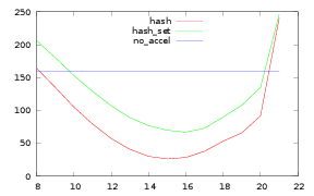
On figure 1, we have the result of the experimentation. The x-axis is the size of the hash table in bits, the y-axis the time needed to solve the 13243 instances. The blue plot is the time without hash tables, the red one the time with a simple array hash table and the green one the time with an array containing sets to hold all numbers.
As expected, the cache issue is a fundamental one, and results are in accordance with the theory. Let’s concentrate on the red plot, which is the easiest to interpret. As long as we remain in the L2 cache (up to 15), increasing the size of the hash table enables to store more elements and thus to cut more branches in the tree. For n=15, the 13243 instances are solved in 26s, 5 times faster than without hash tables. Over n=15, part of the hash table is in the L3 cache and thus, while we are still cutting more branches as we are storing more elements, L2 cache faults are slowing the program faster than we are accelerating it by cutting more branches. For n=20, we begin to have problems to keep the hash table in the L3 cache, and for n=21 there are so many L3 cache faults that the program is slower than what it was without hash tables.
The green plot shows that when we store all results in an array of sets, there are quickly too many elements, and thus we are never able to remain inside the L2 cache. The minimal time is 67 seconds which is the time we also have for n=19 with the simple array structure when we still fit inside the L3 cache. There are however not too many elements as data clearly remain inside the L3 cache as long as the size of the hash array itself is less than the size of the L3 cache. As soon as we are out of the L3 cache, the two methods give the same (bad) results: times are equal for n=21 as most of the time is spent in cache faults.
This might seem like a strange result but the reason is easy to understand: the program is doing very little work between two accesses to the hash table: one arithmetic operation and a few tests, reads and stores. All these operations use data and code that remain in the L1 cache, and they are thus extremely fast. Then, memory accesses can become the bottleneck of the program. Let’s also remember that the number of generated positions with the depth-first algorithm is between 6! 5! (3/2)5=656100 and 6! 5! (4/2)5=2764800, and that we never store the leaves of the tree, which implies that we could store at most around 500000 positions, and we store much less than that, as many generated positions are identical. As 500000 is almost 219, n=21 is overkill anyway.
There is however a lesson to remember here: despite what many people say or write, the larger is not always the better for hash tables. Sometimes, you first have to keep the hash in the cache.
Implementing the breadth first algorithm is not much more complicated than implementing the depth first algorithm. We first need to create a data structure that contains the information needed to build the numbers generated by a subset of the initial pool. For example, we need to know how to build the numbers generated by the first, second and fourth number of pool. In order to do this efficiently, we create an array of list where the i-th element contains the list of pairs of sets to combine in order to build the numbers generated by the subset represented by the binary decomposition of i. This might sound complicated, but is easy to understand with a few examples:
This array of list of pairs can be pre-computed and stored once and for all. The size of the array is 2n−1 where n=6, so the array here has 63 lists of pairs.
The rest of the algorithm is straightforward. Another array of the same size is used, where the i-th element is an array that will hold all numbers generated for the i index.
Let’s see that on an example. If the initial pool of numbers is
{7,8,9,10,25,75} we first copy 7 at position 1, 8 at position 2, 9
at position 4, 10 at position 8, 25 at position 16 and 75 at position
32. Then, all elements with an index having only 1 bit are
filled. Then we fill all elements having an index with 2 bits.
For example, element 3=112 is {7+8,8−7,7×8}={15,1,56},
element 5=1012
is {7+9,9−7,9×7}={16,2,63}, element 6=1102 is
{17,1,72}, and so on. When all elements with a 2-bits index are filled,
elements with a 3-bits index are filled. For example element 7=1112
is
{15+9,15−9,15×9,1+9,9−1,56+9,56−9,56×9} ∪
{16+8,16−8,16*8,16/8,2+8,8−2,8×2,8/2,63+8,63−8,63×8} ∪
{17+7,17−7,17×7,1+7,7−1,72+7,72−7,72×7} =
{24,6,135,10,8,65,47,504,24,8,128,2,10,6,
16,4,71,55,504,24,10,119,8,6,79,65,504}.
There remains a few implementation details to solve. Whether it is better to use an array of arrays or an array of sets is unclear. Both structures have their advantages and their disadvantages. An array has an access time which is constant, while inserting a new number in a set of size n takes logn operations when using a binary balanced tree structure for the set. However, when using sets, duplicates numbers are never kept and there are lot of duplicates: even in the simple example above, there are already many of them in the 3-bits 7th element. Another (minor) advantage of the sets is that they use exactly the right number of elements while the size of arrays has to be pre-computed at allocation time; however this minor point may be circumvented in different ways: first we know a quite good estimate of the size of each array, as the N(p) numbers computed in section 2.3 are an upper bound of the size of a p-bits array. Moreover, it is possible to break the (large) arrays into a list of smaller arrays which are allocated when needed.
Last, but not least, it is important to notice that while all numbers have to be generated (of course), numbers generated by the full set of the original pool (the array element with all bits set to 1) do not have to be stored, as they will never be re-used. It is an extremely important optimization of the code, as they are, and by far, the largest set.
Experimental results with n=6 are the following : the breadth first algorithm with an array-array structures solve the 13243 instances in 53s, and in 89s with an array-set structures. The results of all the algorithms are summarized in table 1.
Algorithm Total Time By instance Depth first 160 12.10E-3 Depth first / hash 26 1.96E-3 Depth first / hash-set 67 5.05E-3 Breadth first / arrays 53 4.00E-3 Breadth first / sets 89 6.72E-3
The most efficient algorithm for n=6 is the depth first algorithm with standard hash tables. The worst is the basic depth first algorithm. Results are in accordance with the complexity analysis done in section 2, as breadth first search is more efficient than depth first search without hash tables. However, it would be extremely interesting to see what happens with higher values of n.
The depth first algorithm with hash tables is extremely efficient. There are other programs available on the net which claim to solve also the complete set of instances such as Fouquet [2010], but in 60 days (!).
Since its beginning in 1972, the numbers round of the Countdown game has never evolved, while its sister game, the letters round, has seriously changed, going from 7 letters in 1972 to 10 letters today. In 1972, computers were enable to solve the numbers round; nowadays, it is solvable in less than a millisecond. So, as in many games where computers have become much better than human beings, the interest for the game has faded. Moreover, the game by itself is not very difficult on the average for human beings4
There are thus two questions: is it possible to modify the game in order to turn it into a difficult thing for a computer, and is it possible to turn it into a game more difficult for the players without modifying it too much?
There are two ways to change the difficulty of the game. The first one is to choose the target number based on the values in the number set, or even to choose only a tuple (numbers set,target value), such as the number of operations for finding the target with the given numbers set is high.
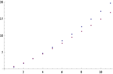
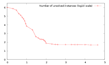
The other idea comes from the complexity study which provides a hint: when the size of the sets of available numbers increases, the game becomes apparently extremely difficult. If we use the complexity formulas of sections 2.2 and 2.3, we plot (figure 2) in blue the log10 of the number of operations required by the depth first algorithm and in red the same quantity for the breadth first algorithm.
The breadth first algorithm quickly becomes much more efficient than the depth first algorithm. However, its space complexity is also increasing at almost the same rate as its time complexity, while the space complexity of the depth first algorithm remains extremely small. But these results do not take into account the hash table effect for the depth first algorithm, or the set effect for the breadth first algorithm, which are both going to become primary factors as the number of duplicate positions and numbers will be much more important as there will be much more ways to compute numbers (especially small numbers) with a larger set of initial numbers. The number of generated numbers is also going to increase: this means that to have a depth first algorithm efficient, the size of the hash tables has to be increased, which will take us out of the L2 and the L3 cache, and thus slow down significantly computations.
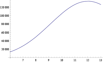
To compute the total number of different instances5, we can extend the formula in section 3:
|
This formula is valid for n≤20 and the number of instances is n(7)=27522, n(8)=49248, n(9)=76702, and n(10)=104753. The results are summarized on figure 3.
For n=6 we have 13243 possible sets. In the standard numbers round of the countdown game, we search for numbers in the range 101–999, so there are 899×13243=11905457 possible problems. In table 2 we have the distance to the closest numbers: 10858746 games are solvable (91.2%), 743896 problems (6.25%) have a solution at a distance of 1 (the nearest number).
distance solved %solved cumulative 0 10858746 91.21% 91.21% 1 743896 6.25% 97.46% 2 100517 0.84% 98.30% 3 36186 0.30% 98.60% 4 19387 0.16% 98.76%
1226 instances out of 13243 (9.2%) solve all target numbers in the range 101-999. One instance ({1,1,2,2,3,3}) solves none.
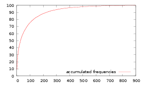
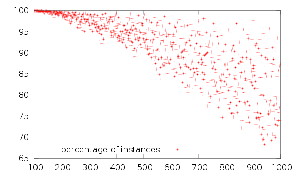
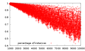
On figure 4, we see that 9998 (75.5%) of the possible instances solve all possible games with less than 100 numbers missing in the range 101–999.
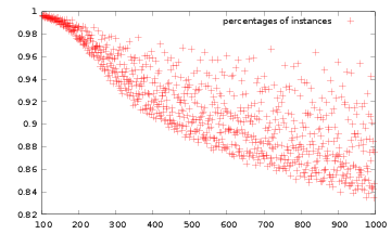
The easiest numbers to find are 102, 104 and 108 which are found by 13240 instances (99.98%). The most difficult number to find is 947, which is only found by 9017 instances (68%).
On figure 5, we see that, as we might have expected, the easiest numbers to find are the lowest, and the most difficult are the highest. Numbers below 300 are all found by 95% of the possible instances.
Another interesting statistic for the player of the British version of the game is how the distribution of large (25, 50, 75, 100) and small (1 to 10) numbers influence the number of solutions available. Each large number is present in C135+C101C123+C102C111=3982 instances (30%) of the 13243 instances, while each small number appear in C135+C134+(C101−1)C123+C91C122 +(C102−C91)C111+C92=5008 instances (38%).
On figure 6, we see the percentage of problems solved when a number x is in the original set.
The worst number is 1 (only 86% problems are solved when 1 is in the set) and the best is 75 (almost 96% are solved when 75 is in the set). But the differences are not that important between large and small numbers: for x=9, 93.5% are solved, not that far from the 94.2% for x=25.
In table 3, we see how the number of large numbers in the set influences the resolution. For example there are C106+ C101C94+ C102C82+ C103=2850 instances with no large numbers, and thus 2850*899=2562150 problems and 1963762 of these problems can be solved (77% success rate).
nb large problems solved %solved 0 2562150 1963726 77% 1 5221392 4966076 95% 2 3317310 3192103 96% 3 755160 693131 92% 4 49445 43710 88% 11905457 10858746 91%
The influence of large numbers is much more visible here. Instances with 1–3 large numbers have a success rate of 92–96%, and even with the four large numbers (25,50,75,100) the success rate is higher that with none of them. However, the importance of large numbers must not be overestimated, as Tunstall-Pedoe [2013] does. The 4-tuple (25,50,75,100) has a success rate of 88%, much less than (5,7,9,100) which has a success rate of 99.86% and contains only one large number (the worst 4-tuple is (1,1,2,2) with a success rate of 37%).
There is another site (Lemoine and Viennot [2012]) in french which advertises the kitsune program and gives some stats. However, it takes a few hours to compute them, while this program takes only a few seconds. So, for the fans of statistics and results, here are some other “funny” facts:
As all instances have been solved, we have a complete database; for a given number set and a given target number we know if it can be solved and how many operations are necessary to solve it, or how close is the nearest findable number when it can’t be solved. With this database, it is extremely easy to select only interesting problems. There can be many different selection criteria: solvable problems requiring more than 4 (or 5...) operations, or unsolvable problems with the nearest number at a minimal given distance, or unsolvable problems with the nearest number requiring more than 4 operations, etc… This would turn the number round in something worth watching again.
Another way to make the game harder would be to use all available numbers between 1 and 100 when picking the set. Building the full database is much more computing intensive. In the standard game we have 13243 sets, when picking k numbers between 1 and n (including repetitions) we have Cn+k−1k=C100+6−16=1609344100≃1.6 109 possible sets, and 1446800345900≃1.4 1012 problems. Building the database took 12 hours on the cluster described in section 3.
Table 4 gives the distance to the solution, as table 2 does for the standard game. Percentages are similar to the standard problem.
dist solved %solved cumulative 0 1329106855477 91.86% 91.86% 1 105091143229 7.26% 99.12% 2 8508187551 0.59% 99.71% 3 2112923902 0.14% 99.85% 4 808768195 0.06% 99.91%
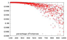
In figure 7, we have the same results as in figure 5. Percentages are higher which means that on the average, the problem is easier to solve with numbers picked randomly between 1 and 100.
There are 73096123 (4.5%) sets that solve all problems. This is less in percentage (1226/13243≃9.2%) than for the standard game, but there are 60000 times more sets if we consider the raw numbers. So we can select some sets with specified characteristic that would make them difficult for human beings, while maintaining the diversity of the problem. There are for example 52253 sets that solve all problems while being composed only by prime numbers, 48004 by primes ≥ 2, 22136 by primes ≥ 3, 8912 by primes ≥ 5, 4060 by primes ≥ 7, 1526 by primes ≥ 11, 500 by primes ≥ 13, 132 by primes ≥ 17, and 4 by primes ≥ 23. As incredible as it might look, the set {23,29,31,37,43,61} solves the 899 problems.
Another criteria could be to select sets where all numbers are greater than a given one; there are for example 20602 sets with all numbers >25 that solve the 899 problems. The set {35,37,38,43,45,59} is one of them…This method can be combined with the one described in section 4.1.2, by choosing only target numbers that require a minimum number of operations. Here again, the possibilities are endless, and it would turn the numbers game into something really difficult while always using 6 numbers.
Using equations 1, 2, 3 and 4 we find that the maximal and minimal number of operations for the depth first algorithm are dmax(7)=232 243 200 and dmin(7)= 41 334 300. For the breadth first algorithm, we have bmax(7)= 49 951 531 and bmin(7)= 9 379 195. We thus have dmax(7)/dmax(6)=84, dmin(7)/dmin(6)=63, bmax(7)/bmax(6)=43, bmin(7)/bmin(6)=32.
In table 5 we have the results of the experimentation with the five algorithms with n=7.
Algorithm Total Time By instance Depth first 740 740E-3 Depth first / hash 36 36E-3 Depth first / hash-set 114 114E-3 Breadth first / arrays 109 109E-3 Breadth first / sets 131 131E-3
We see that with the depth first algorithm, the time for solving instances with 7 numbers is 62 (740/12) times larger than with n=6. This is completely compatible with the minimal complexity of this algorithm, which predicts a ratio of 63.
With the breadth first algorithm, the time for solving instances with 7 numbers is 28 (109/4) times larger than with n=6. This is slightly less than what was expected (a ratio of 32) but remains in line with what was expected.
With the depth first algorithm with hash table, the ratio is only 18. Hash tables are getting more and more efficient, as small numbers are generated more often. An analysis of the optimal size of the hash table shows that the best size is around 219 instead of 215 for 6 numbers: more space is needed to hold more numbers, even if data can not remain inside the L2 cache.
Regarding the resolution of problems we see on figure 8 how numbers are found.
With an extra number in the set, the success rate becomes extremely high. All numbers are found by at least 98.5% of the instances: the problem has become too easy.
If we try to find numbers in the range 1000–10000 instead of 100–1000, we see on figure 9 that the problem is now too difficult.
The right solution is to look for numbers in the range 1000–6000 (the most difficult number to find is then 5867, with 65% instances finding it) . The success rate is now almost the same as what it was with 6 numbers in the range 100–1000, but with a resolution time which is 20 times higher. However, the solution of a problem is found by the best algorithm in 36 milliseconds, which is still much too fast to put the machine in the same league as a human being…
We have here bmin(8)= 363 099 899, dmin(8)= 3 472 081 200 and dmin(8)/dmin(7)=84 and bmin(8)/bmin(7)=39.
In table 6 we have the results of the experimentation with the five algorithms with n=8.
Algorithm Total Time By instance Depth first 610 61 Depth first / hash 12 1.2 Depth first / hash-set 37 3.7 Breadth first / arrays 44 4.4 Breadth first / sets 41 4.1
We see that with the depth first algorithm, the time for solving instances with 8 numbers is 83 (61/0.740) times larger than with n=7. This is completely compatible with the minimal complexity of this algorithm, which predicts a ratio of 84.
With the breadth first algorithm, the time for solving instances with 8 numbers is 40 (4.4/0.109) times larger than with n=7. This is exactly what was expected (a ratio of 39). We notice that the breadth-first-set algorithm is becoming faster than the breadth-first-array algorithm. With 8 numbers, we are generating more and more small duplicate numbers, and thus the time lost with the logn access for sets is now compensated by the time gained with the elimination of all these duplicates numbers. With the depth first algorithm with hash table, the ratio is 33. The memory needed to run the breadth-first-array algorithm is 1.5Gb. The breadth-first-set algorithm still has small memory requirements. For the depth-first with hash, the optimal value of the size of the hash table is around 223 elements.
The results are presented in figure 10. Computation took a few hours.
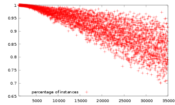
There again, with an additional number, the problem becomes too easy to solve in the previous range (1000–10000). The correct range must be extended up to 35000 as we have then roughly the same mean success rate as with the standard game (the most difficult number to find is 34763 with a success rate of 66%). However, if the depth first program is now unable to compute the solution in less than 30s (English game) or 45s (french game), the depth-first with hash still finds a solution in 1.2s on the average.
We have dmin(9)/dmin(8)=108 and bmin(9)/bmin(8)=48. Thus the standard depth first algorithm should take more than 6000s to solve a single instance and the breadth first algorithm with arrays should need around 40Gb of memory, that the computer used for these tests don’t have.
In table 7 we have the results of the experimentation with three algorithms with n=9. The depth first algorithm wasn’t, as expected, able to solve even a single instance in less than 1 hour. The breadth first algorithm with arrays generated an “Out of memory” error.
Algorithm Total Time By instance Depth first - - Depth first / hash 147 14.7 Depth first / hash-set 543 54.3 Breadth first / arrays - - Breadth first / sets 467 46.7
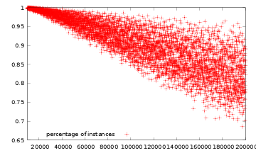
The results are presented in figure 11.
We have to extend the range up to around 200000 (the most difficult number to find is 190667 with a success rate of 66%). Computing complete results took 3 days.
For n=10 we are at last entering uncharted territory. The average time to solve one instance of the problem seems to be around 1 to 3 minutes, so it seems impossible to use an exhaustive algorithm. We are at last back in the heuristics land.
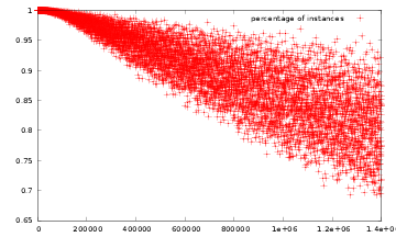
The results are presented in figure 12.
Complete results were computed in 20 hours on the cluster described in section 3. Some pools such as {5,6,7,8,9,10,25,50,75,100} took more than one hour to complete. We had to extend the range over 1000000 to have similar results regarding success rate (up to 1000000 the most difficult number to find is 986189 with a 67% success rate).
The problem is easy to solve because it is a finite one: at each step, the set of available numbers is reduced by one unit, and thus any computer program can solve it even with a very large set of numbers. An other solution to turn the game into a more interesting one would be to add a simple operation: the possibility to replace any available number by its square.
Let’s see this on an example: how to find 999 using {1,2,3,4,5,6}. This is an unsolvable problem without the square operation, but it is now not the case anymore:
   Operations     Remaining
  3 x  6 =  18  {1,2,4,5,18}
 18 x 18 = 324  {1,2,4,5,324}
  4 +  5 =   9  {1,2,9,324}
324 +  9 = 333  {1,2,333}
  1 +  2 =   3  {3,333}
333 x  3 = 999  {999}
This modification changes the nature of the game, because it is not any more a “finite” one, at least in theory. Thus, we can have long and complex computations to find results. Let’s see it on an example: how to find 862 using the {1,10,10,25,75,100} set. The shortest computation requires 14 steps (while in the standard game we can never have more than 5 steps) and uses very large numbers:
{1,10,10,25,75,100}
10 - 1 = 9
{9,10,25,75,100}
100 x 100 = 10000
{9,10,25,75,10000}
9 x 9 = 81
{81,10,25,75,10000}
10 x 10 = 100
{81,100,25,75,10000}
100 x 100 = 10000
{81,10000,25,75,10000}
10000 + 10000 = 20000
{81,20000,25,75}
75 x 75 = 5625
{81,20000,25,5625}
5625 x 5625 = 31640625
{81,20000,25,31640625}
20000 x 20000 = 400000000
{81,400000000,25,31640625}
400000000 - 31640625 = 368359375
{81,368359375,25}
25 x 25 = 625
{81,368359375,625}
625 x 625 = 390625
{81,368359375,390625}
368359375 / 390625 = 943
{81,943}
943 - 81 = 862
The program has to be slightly modified to include the possibility to raise a number to its square at any time, and it must also be limited: we have to set an upper bound A above which we do not square numbers anymore. Without this bound, the algorithm might not stop. Moreover, because of implementation issues, the maximal value of A that can be tested with 64 bits arithmetic is 45000.
The possibility of squaring numbers seriously increases the complexity of the program. As we are only interested in finding whether a given set is able to solve all numbers in the range 101–999, we stop as soon as all these numbers have been found and do not keep on searching for the shortest solution available. With this optimization, and by using all the other optimizations presented above, computation time is not really an issue, at least for values of A up to 50000.
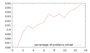
We see in table 8 results for different values of A.
A Sets Instances % unsolved 1 12017 1046711 8.79% 2 10757 758822 6.37% 3 9059 503409 4.22% 4 6275 196070 1.65% 5 5004 128631 1.08% 6 3507 74137 0.622% 7 2478 48932 0.411% 8 1637 29165 0.245% 9 926 13889 0.117% 10 593 7231 0.0607% 20 294 2706 0.0227% 30 99 443 0.00372% 40 55 311 0.00261% 50 41 225 0.00189% 60 40 221 0.00185% 70 35 206 0.00173% 80 31 166 0.00139% 90 28 130 0.00109% 100 20 77 0.000647% 200 17 62 0.000520% 300 16 55 0.000461% 400 16 54 0.000454% 2000 16 54 0.000454% 3000 15 53 0.000445% 4000 14 52 0.000437% 10000 14 51 0.000428% 20000 13 49 0.000412% 45000 13 49 0.000412%
For A=1 the results are the results of the standard algorithm, because squaring 1 gives 1: 1046711 instances (of 11905457) are not solve, and there is at least one number not found for 12017 sets of numbers. The number of unsolved instances reduces quickly in the beginning of the curves, but then slows down.
The results are presented graphically in figure 13.
The 49 instances not solved (with A=45000) are the following ones:
1 1 10 10 25 100: 858
1 1 10 10 25  75: 863
1 1 10 10 50 100: 433 453 547 683 773
                  853
1 1 10 10 50  75: 793 853 978
1 1 10 10 75 100: 433 453 457 478 547
                  618 653 682 708 718
                  778 793 822 853 892
                  907 958 978
1 1 10 25 75 100: 853 863
1 1 10 50 75 100: 793 813 853 978
1 1  5  5 25 100: 813 953
1 1  7  7 50 100: 830
1 1  8  8  9   9: 662
1 1  9 10 10 100: 478 573 587 598
1 1  9  9 10 100: 867
1 9  9 10 10 100: 867 947 957 958 967
If searching for results in the range 1001–9999 instead of 101-999, the percentage of solvable problems remains extremely high (at least 99.9705%: only 35200 instances out of 119173757 seem to be unsolvable). However problems are usually much more difficult for a human being, as they require using much larger numbers. Another interesting proposal to revive the current countdown game would be to keep on using 6 numbers drawn in the same pool, but to search now for numbers in the range 1001-9999 and to allow using the square operation.
From a theoretical point of view, the main question is: are there some instances that can never be solved whatever the value of A?
This question is a complex one and requires further research: on the one hand, we can hope that by searching with large enough values of A we would solve all instances of the problem. However, if our search is not successful, it is pretty much unclear how to demonstrate that a given instance has no solution. This could indeed be an example of a simple undecidable problem.
When looking for a specific number there are often many different ways to find the result. However, most of these solutions are “identical” from a human point of view. There are unfortunately no clear boundary between “identical” and “different” solutions. There are some elementary rules that can be used to reduce the number of solutions, but it is highly improbable that the filtered solutions would satisfy all fans of the game.
We use postfix notation (A+B will be written (+ A B)) as any computation can be written as a tree and filtering solutions is therefore nothing more than tree reduction. Here are the rules that were used to reduce the tree:
These rules have to be applied until the tree is stable.
The results are presented in figure 14.
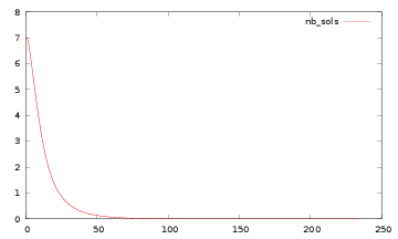
833814 problems (7%) have 1 solution, 800633 (6.72%) have 2 solutions, etc…The largest number of different solutions is 232 when the set is {2,4,5,6,10,50} and the number to find is 120.
Tu turn the problem into a challenging one for a human being, this article proposes different solutions which are easy to use. As the game has been completely solved for n=6, both with the standard set of numbers and with the extended set of all numbers from 1 to 100, it is easy to pick numbers and target such that the problem is challenging for a human being, either by choosing problems which require a minimal number of operations, or unsolvable problems with the best findable number at some distance of the target, or using sets having only prime numbers or large and “unfriendly” numbers. Another solution would be to use more than 6 numbers, and to use a target in a range above 1000, but it is probably not necessary. The last solution is to change a little bit the game by adding the square operation. We have proved that it is possible with only 6 numbers to find the exact solution for 99.9705% of the problems with the target in the 1001–9999 range. This is however much more difficult for a human being, because using the target is higher, and the square is not a natural operation to use.
It is more difficult to turn the game into a challenging problem for a computer. While the classical depth-first algorithm fails to find a solution in the allotted amount of time for n>7, our algorithm solves the problem with up to 9 numbers in the set. The n=10 problem is out of reach for an ordinary computer. It would however be interesting to start a challenge between computers for n=10, or n=11 to see what heuristics methods are the best for solving this problem. Using the square operation change fundamentally the problem from a theoretical point of view, because the game might be undecidable. Proving the undecidability remains an open challenge, and finding solutions for the currently unsolved problems (49 instances for the standard set of numbers and standard target) is still open.
This document was translated from LATEX by HEVEA.
This page has been read
times (in english or in french).